Lab 04: Gyro Modeling and Control

Lab Overview

Course: AE 443 – Experimental Dynamics and Control Laboratory (Bernardo Restrepo / Jared Getz) | April 10, 2026
Objective: Model the open-loop rotary gyroscope dynamics, design a PI controller to track a 2° deflection reference angle α, and compare open-loop vs. closed-loop disturbance rejection. Validate stability using the Routh-Hurwitz criterion.
Open-loop model: α(s)/V_m(s) = (1/G_g) · K/(τs+1) where K = 1.53 rad/s/V, τ = 0.9 s, G_g = 5.20 1/(rad·s)
Closed-loop TF: G_CL(s) = K(sk_p + k_i) / [G_gτs² + (Kk_p + G_g)s + Kk_i]
Hardware: SRV02 with rotary gyroscope attachment, Q2-USB DAQ

Open-loop alpha response (Fig. 1)

Open-loop theta response (Fig. 2)

Open-loop voltage response (Fig. 3)

PI Controller Design & Analysis

The PI controller law V_m(s) = (k_p + k_i/s)·e(s) was substituted into the open-loop gyroscope model to derive the closed-loop transfer function G_CL(s). Matching its denominator to the standard second-order form s² + 2ζω_ns + ω_n² gave the gain expressions:

k_p = G_g(2ζω_nτ − 1) / K k_i = G_gτω_n² / K

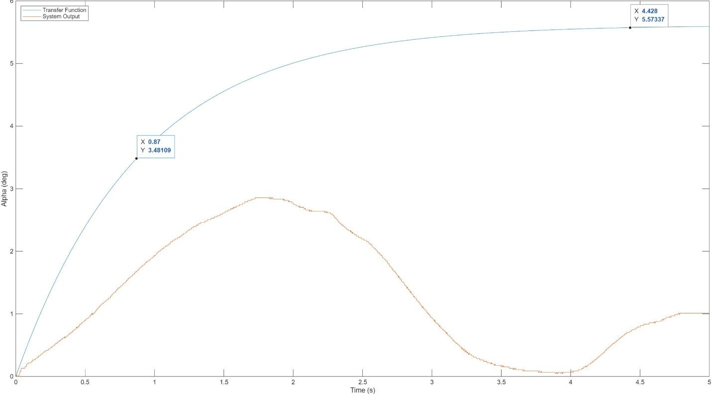
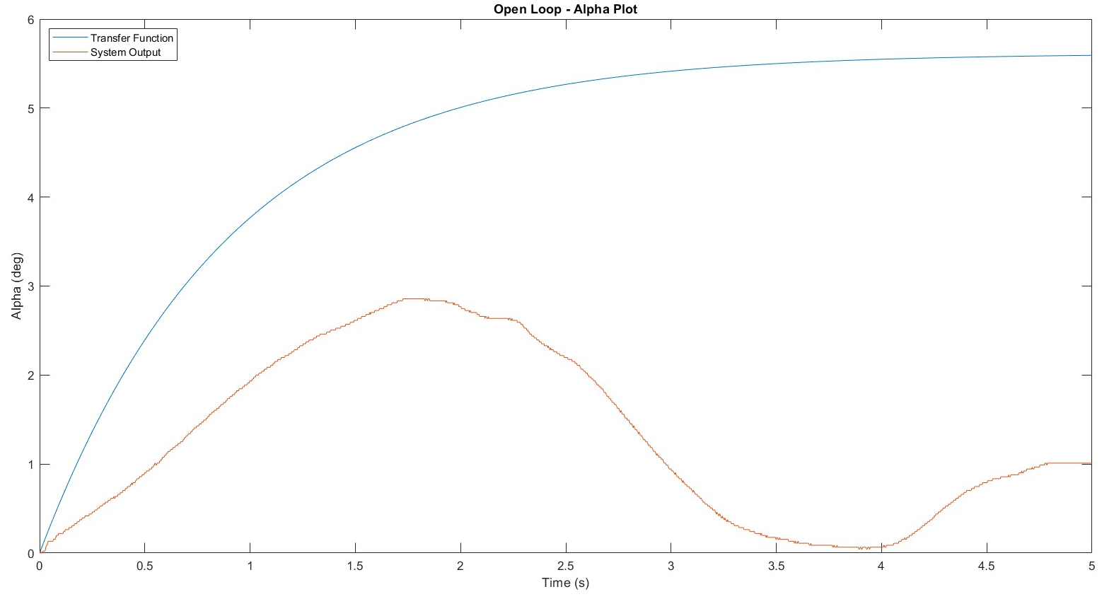
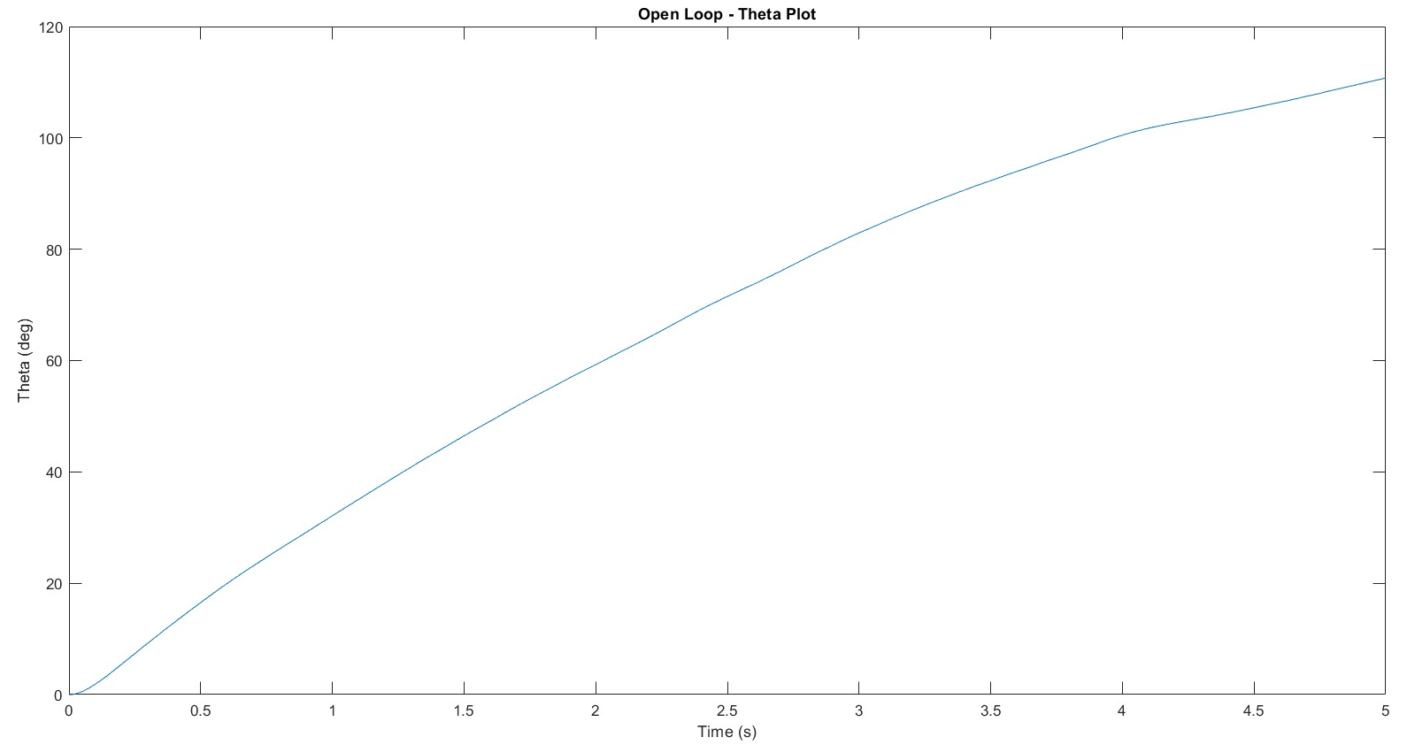
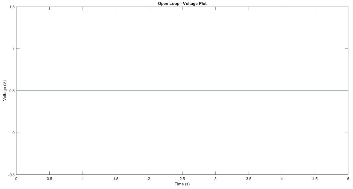
Using ζ = 1.05 (slightly overdamped), ω_n = 3.61 rad/s, and the system parameters: k_p = 19.79, k_i = 39.86. The experimental open-loop time constant was identified as τ = 0.87 s using the 63.2% criterion on the α step response. The open-loop model predicted α_ss = 8.43° but measured only 2.8° (66.8% error), explained by unmodeled gyroscopic coupling and sensor noise.

Closed-loop alpha tracking 2° (Fig. 4)

Closed-loop voltage response (Fig. 6)

Disturbance response — PI on (Fig. 7)

Results: Closed-Loop & Disturbance Rejection

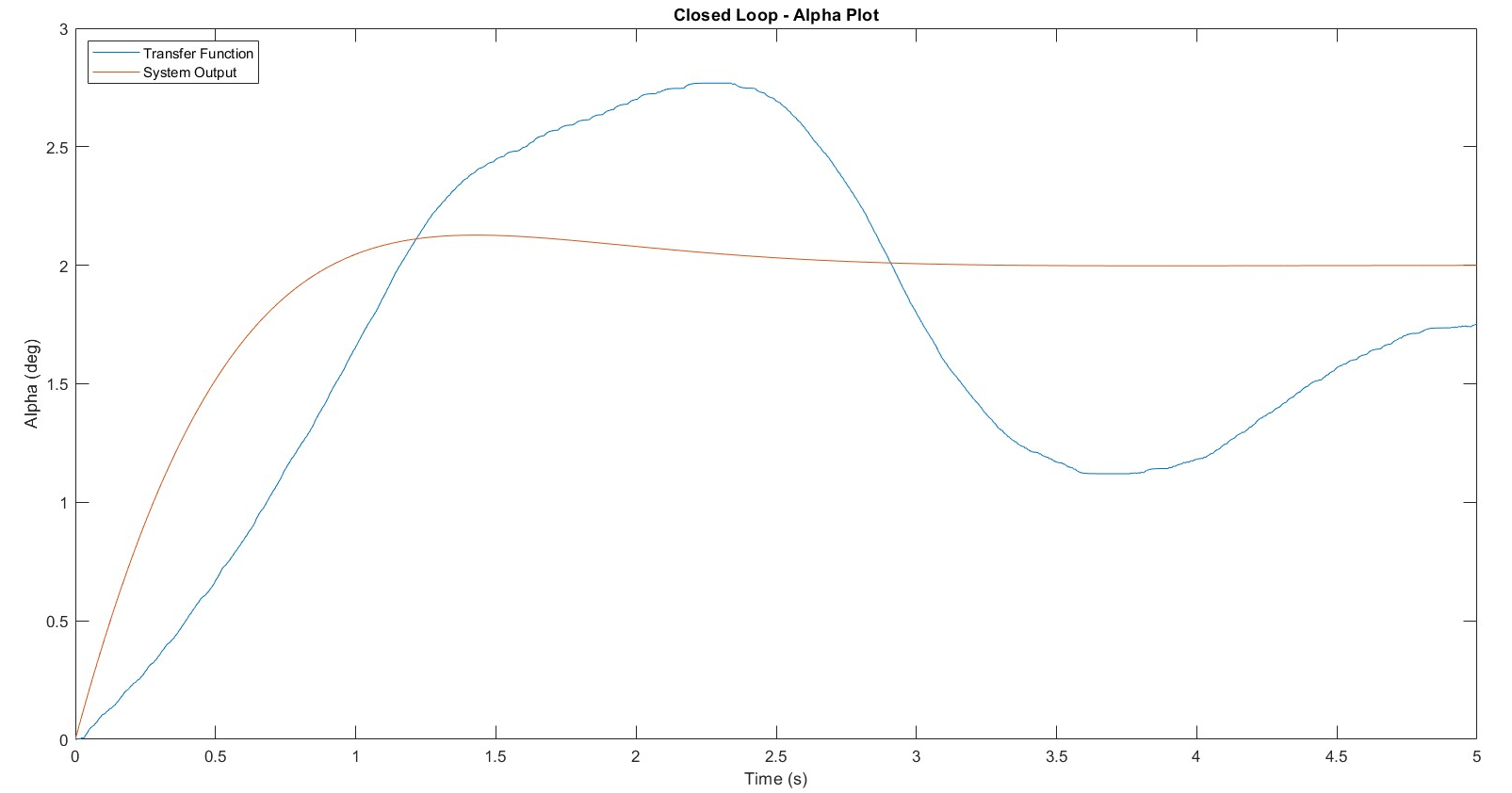
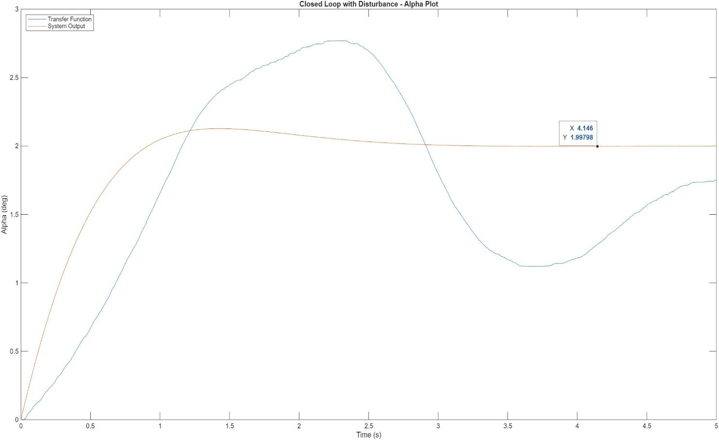
Closed-loop tracking: With PI control, α converged to 1.997° (e_ss = 0.003° ≈ 0), confirming the integral action eliminates steady-state error for a step reference input.
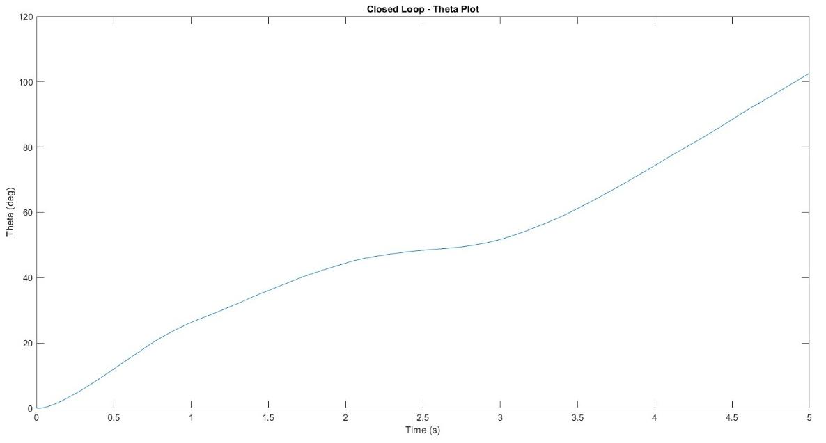
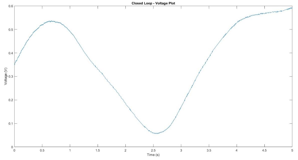
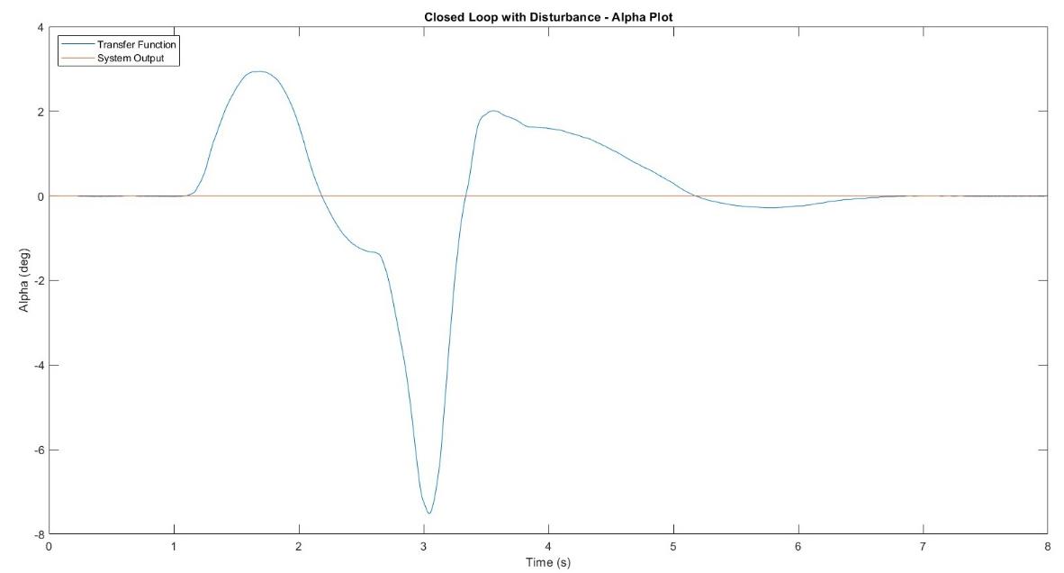
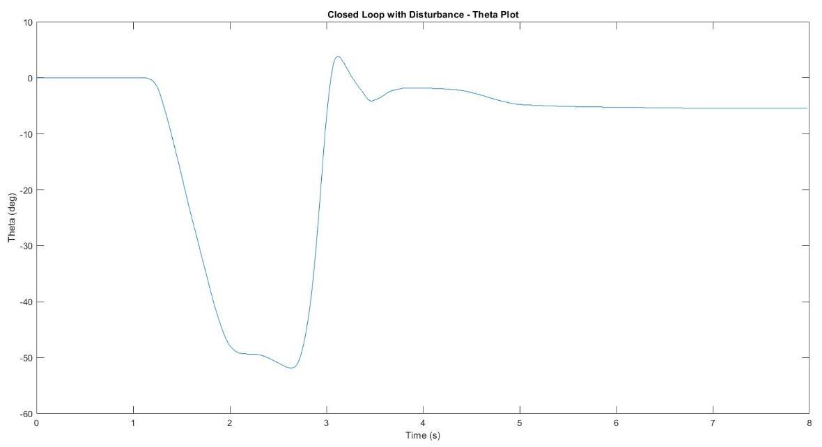
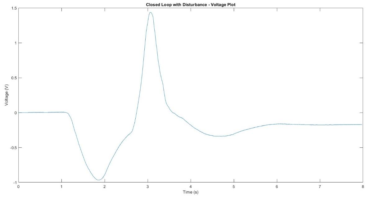
PI control ON — disturbance: Motor voltage adjusted dynamically to oppose base rotation; servo angle compensated rapidly; α remained at ≈0° (e_ss = 0°), demonstrating active disturbance rejection.
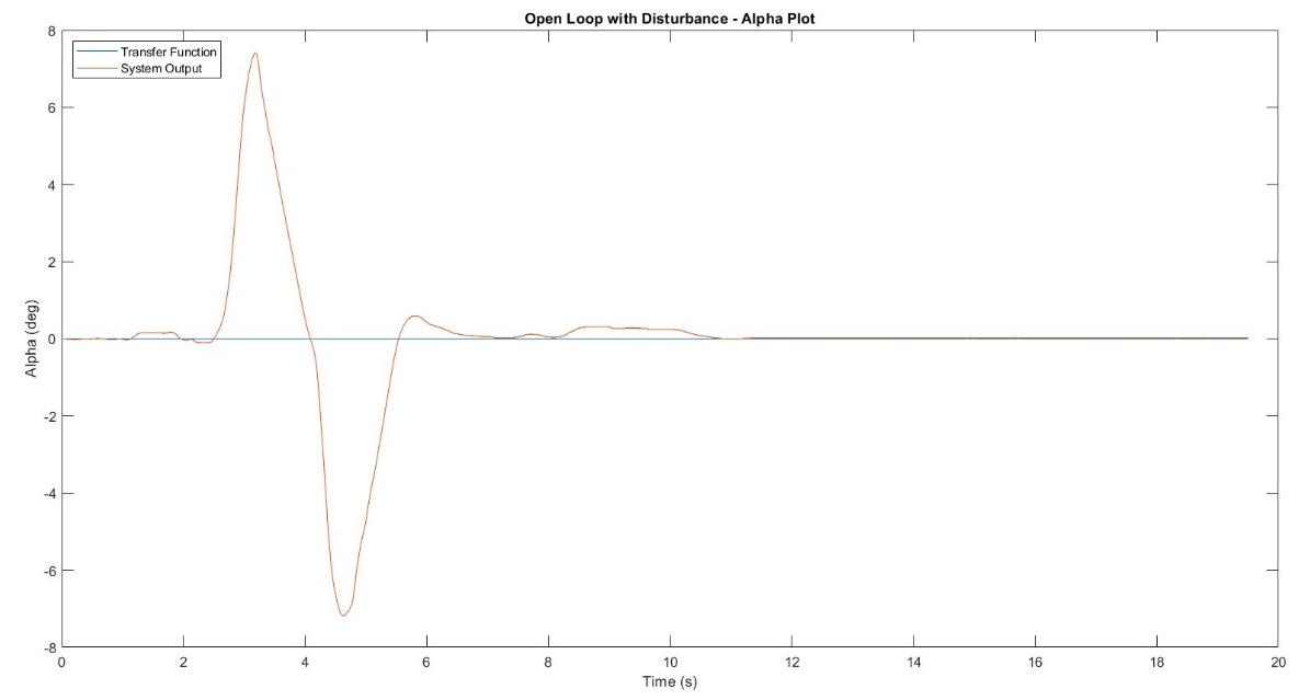
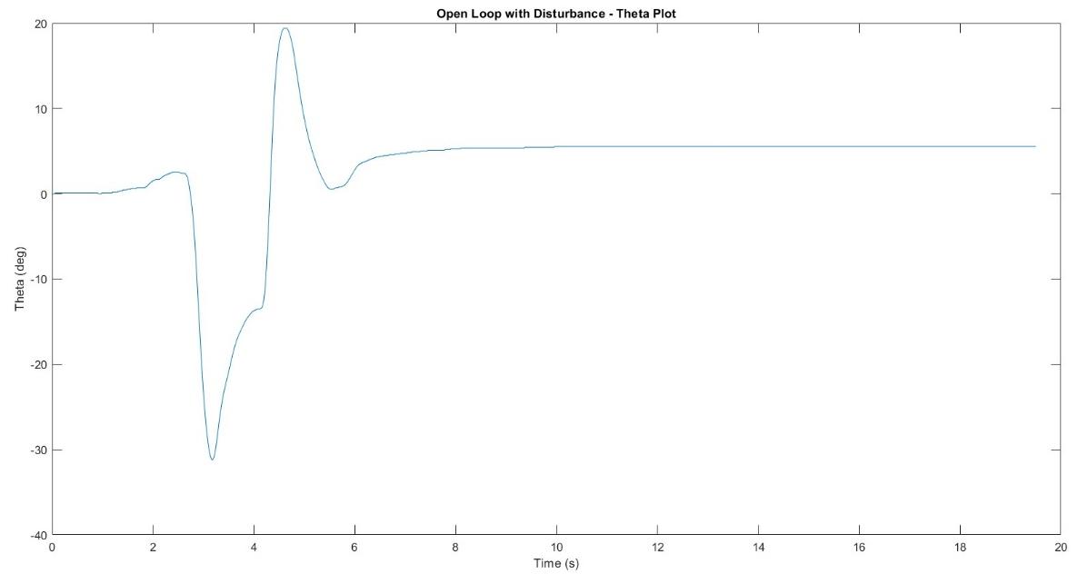
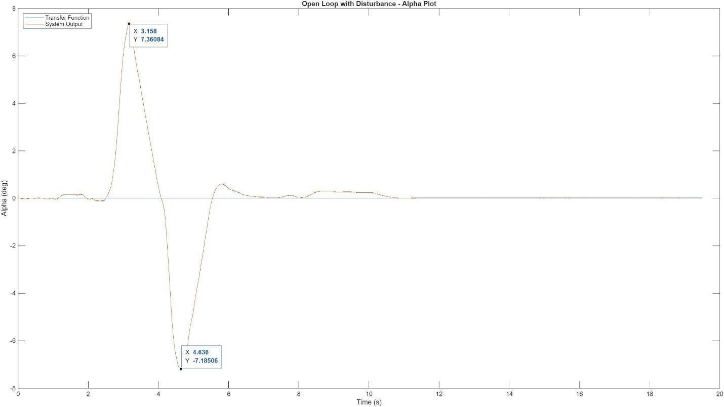
PI control OFF — disturbance: Motor voltage = 0; deflection reached ±7.4° before passively recovering over ≈20 s. Gyroscope heading was not maintained without feedback.
Routh-Hurwitz (open-loop): Single pole at s = −1/τ = −1.11 → left-half plane → stable.
Routh-Hurwitz (closed-loop): All three Routh table entries positive for k_p = 19.79 > −3.40 and k_i = 39.86 > 0 → closed-loop system stable.
The gyroscope must continuously rotate about the z-axis to sustain a non-zero α, reflecting the physics: T_g = H·θ̇, so a constant deflection requires constant base angular velocity.

Open-loop disturbance — alpha (Fig. 10)

Closed-loop alpha converged to 2° (Fig. 13)

Routh-Hurwitz table (Table 1)

MATLAB Code

Separate figures were generated for open-loop and closed-loop responses of α, θ, and V_m, overlaying transfer function predictions against measured hardware data. Full script: Lab 4 Appendix A.

% Open-loop alpha plot with TF overlay
figure()
plot(data_alpha(:,1), data_alpha(:,2))   % transfer function prediction
hold on
plot(data_alpha(:,1), data_alpha(:,3))   % measured system output
xlabel('Time (s)');  ylabel('Alpha (deg)')
title('Open Loop - Alpha Plot')
legend('Transfer Function', 'System Output', Location='northwest')

% Closed-loop with disturbance — PI ON
figure()
plot(data_alpha_PI(:,1), data_alpha_PI(:,2))   % TF
hold on
plot(data_alpha_PI(:,1), data_alpha_PI(:,3))   % measured
xlabel('Time (s)');  ylabel('Alpha (deg)')
title('Closed Loop with Disturbance - Alpha Plot')
legend('Transfer Function', 'System Output', Location='northwest')

Full MATLAB script — Lab 4 Appendix A

PI controller Simulink block

Gyroscope hardware setup